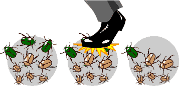
Did you have to Google what genetic drift was before reading this article? I bet you did. Not many people know about this evolutionary mechanism, or even the fact that evolution has mechanisms other than natural selection. In fact, outside of more formal scientific literature, the terms ‘evolution’ and ‘natural selection’ are used interchangeably.

Evolution is actually a collective term for three biological mechanisms that can affect the genetic makeup of populations: natural selection, genetic drift, and gene flow. Natural selection is obviously the most famous, to the point where even those who haven’t taken a science class have some understanding of it: organisms with better genes have a better chance of survival, and therefore a better chance at reproduction, meaning that their genes are passed on to the next generation, leading to organisms best suited to survive in their environment.

With all the attention that natural selection gets, it’s siblings, genetic drift and gene flow, are often left in the shadows. I won’t talk too much about gene flow, the effect of phenotypes moving across different populations, but I will explain the subject of my simulation, genetic drift.

Genetic drift generally occurs in small populations, and ones where differing phenotypes have little to no effect on survival and/or reproduction. A low survival rate also contributes to genetic drift. In these sorts of populations, the effect of randomness is much more permanent; in a large population with a high survival rate, a bunch of organisms of one phenotype dying would have little effect on the population as a whole and would be averaged out by a similar opposite event, due to the law of large numbers. However, in a small population with a low survival rate, this could have a drastic effect on the future of the population as a whole.

For the biology unit in our science class, we had to create either an experiment or design related to biology. I decided to do a design, and to try out a field called bioinformatics, which combines biology with computer science and statistics to analyze and interpret biological data, as well as simulate biological processes. After much looking, I came across the concept of genetic drift, and decided it would be interesting to create a simulation of its effect on populations.

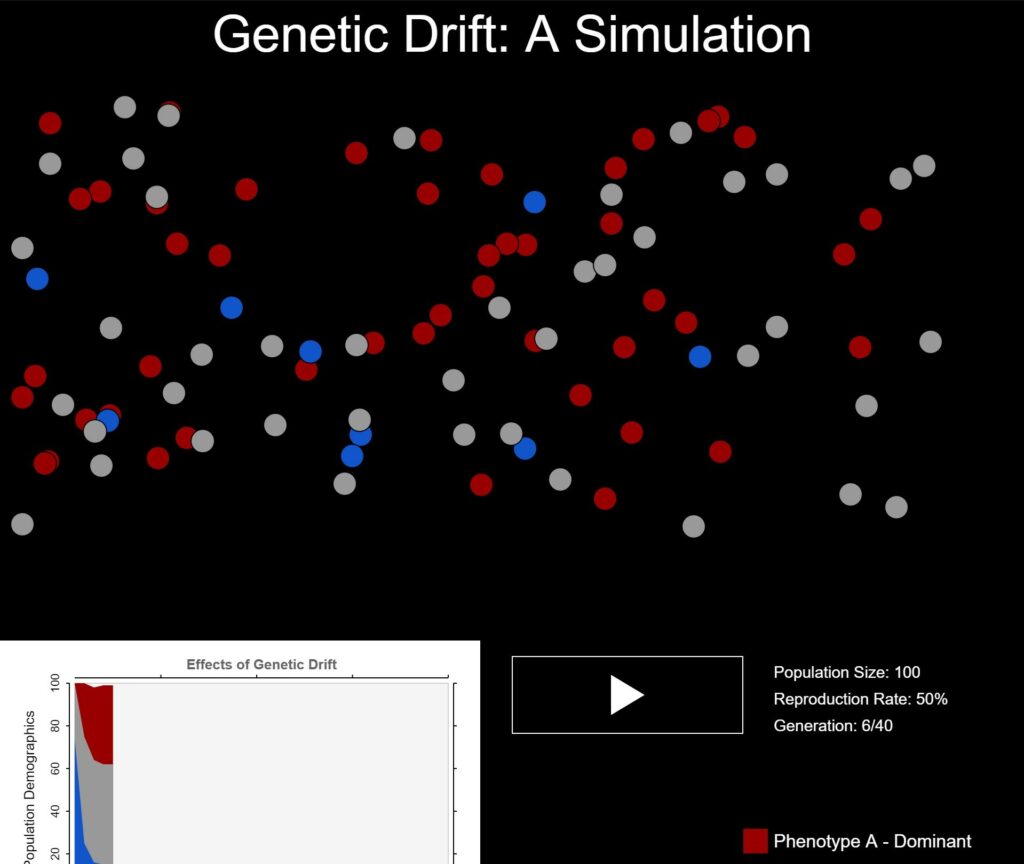
I began by creating a purely numerical simulation that would take a starting population object as input(with the number of organisms in the population with certain phenotypes as values) and returned an array of such objects, representing every successive generation. This didn’t take very long, but I couldn’t really make much of the simulation’s effectiveness in this, form, and an array of objects isn’t very aesthetically pleasing. So I also created a visual using p5, which displayed the number of organisms of each phenotype as colored circles and allowed the user to cycle through generations. I also added a graph that shows how the population progressed.

However, this visualization revealed an error. Rather than trends towards homogeneity, as is expected for a population undergoing genetic drift, the simulation instead stagnated, as shown by this graph.

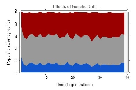
At first, I was confused about the source of this error, and believed it to be an issue in the algorithm itself. However, I soon discovered this issue was occurring because rather than repeat the algorithm for each subsequent generation, I was simply running the algorithm on the first generation over and over again. This is why the demographics stagnated, with very little variance reflecting the randomness in the program.

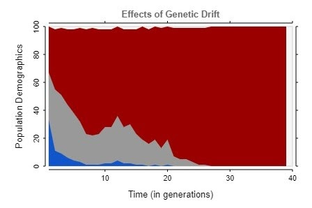
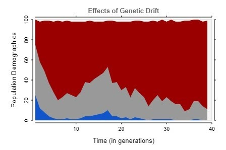
After fixing this issue, the simulation began to show more realistic results, trending towards complete homogeneity in almost every case, as shown by these graphs.

Aside from my recent IDS project, it has been a while since I’ve done a quick and fun programming exercise like this, and in the end, I both sharpened my developing skills and learned more about evolutionary biology.

You can try out the simulation for yourself by clicking this link.